
This post is exclusively an afterthought, as it doesn't really fit well into the main flow of the segment. However, after most models/projects, the final key step is to assess, and if necessary, correct your model and rinse and repeat.
But that really only works well for predictive data. For example, say you beat a multiple regression model for determining the probability that a field goal kick will go in, or for who will win the NCAA tournament, and you insert all the variables you want (kicker, distance, weather, etc; points for, points against, RPI, etc). Well, naturally, you would put in data from this most recent season/tournament, and see how accurately your model predicts the results.
Only that we can't do that here. So you see the rankings of the teams. Now what? Are they wrong? Are they right? I don't know. So what can we do? Throw our hands up in the air and say we can't do anything? No: it's always (sometimes) better to do something bad than nothing at all. So here's something bad:
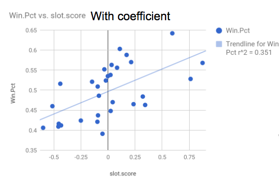
On the X-axis you have every corresponding team's per-pick slot-score average (with coefficient). And on the Y-axis you have every team's winning percentage from 1985 to 2015 (the scope of our data set evaluating draft picks).
With r over 0.59, there is most definitely a correlation -- a mild-to-strong one, in fact -- between the two variables. Here's only a couple -- of the very many, in fact -- reasons why this is indeed "something bad" in terms of assessing our model:
1. Starting with the obvious: there are so many countless variables that go into a team's winning percentage. "How well you performed with the draft picks that you got" might not even crack the top ten. Think of the Knicks: they ranked in the top five, even though their winning percentage was hurt due to trading away several of their first-rounders (which hardly hurt their evaluation in our rankings, as aforementioned). Thus we never really expected the two variables to correlate well at all; it's not like our model was bad simply because r isn't that close to one on this graph.
2. Less obvious: we cannot even establish a causal relationship between "how well you performed with the picks that you had" and "winning percentage" at all. Why? Because "front office competency" could very well be a confounding factor: teams that select well likely have competent front offices, who will in turn make other good decisions, helping the team's winning percentage.
So why did we do this at all, if it's such a terrible measure of how accurate our model is?
Because for us, it wasn't.
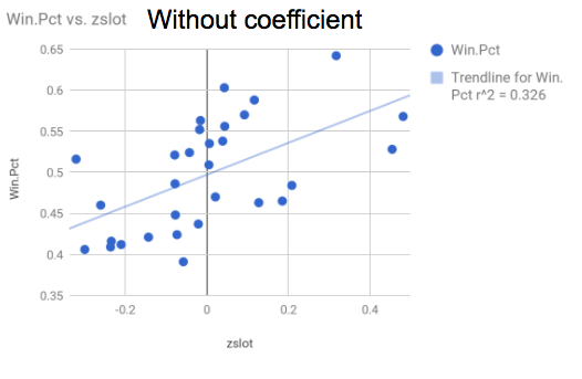
Here is the same graph, only that now the X-axis is the teams' per-pic averages of the z-scores (without the coefficients). Notice how r is now equal to (square root of 0.326) 0.57 -- a weaker correlation than before?
And before we added the ghosts? And adjusted for draft-day trades? R was far lower, down in the 0.30's and 0.40's.
Now, I wouldn't be a good statistician if I told you that I knew that this meant something. So luckily, I'm not: this does mean something (probably)! As we improved our model, the correlation between the teams' rankings and their winning percentage got better. Now, that correlation itself doesn't really mean anything unless you interpret it incorrectly (beware: very easy to do!), but it's rising/falling seemed to be some sort of magic eight-ball for us throughout this project that told us how we were doing, if you follow.
Other ways to evaluate our model? Well, you can have a look at the "best" and "worst" fifteen draft picks above and try to make sense of them, but that's even less scientific than what I just wrote about. You could also possibly compare our final rankings to the "read more" list that I posted the links for above, but we have no guarantees that:
A) those other people were flawless
B) they did a perfectly comparable analysis to ours (well, they didn't)
So again, at the end of the day, we don't really know. That's a lot of what statistics is. It's much easier to disprove things and say that something is wrong than to control for every single possible factor and boil it all down to get exactly what you want. That's why we have things like confidence intervals, and we say things like "correlation is not causation" even it appears on the surface to be the case (the "win % vs. ranking" is a perfect example).
Because sometimes, admitting that you don't know is the most knowledgeable thing to do.
 RSS Feed